MS Excel Part-I – PSEB Solutions

PSEB 9th Class Computer Notes Chapter 1 MS Excel Part-I

November 10, 2021November 9, 2021 by Bhagya

This PSEB 9th Class Computer Notes Chapter 1 MS Excel Part-I will help you in revision during exams.

PSEB 9th Class Computer Notes Chapter 1 MS Excel Part-I

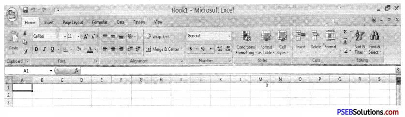
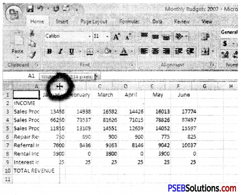
Excel is Product of Microsoft:

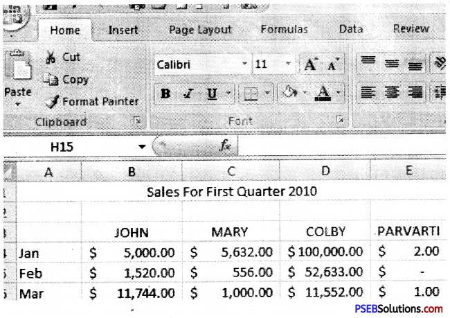
An Excel Workbook consists of many worksheets to perform these calculations. A worksheet is made up of Rows and columns. Intersection of a Row and Column generate a cell.

Formatting Cells:

Each cell in a worksheet can be formatted. Changing the format of a cell doesn’t affect the cell value.
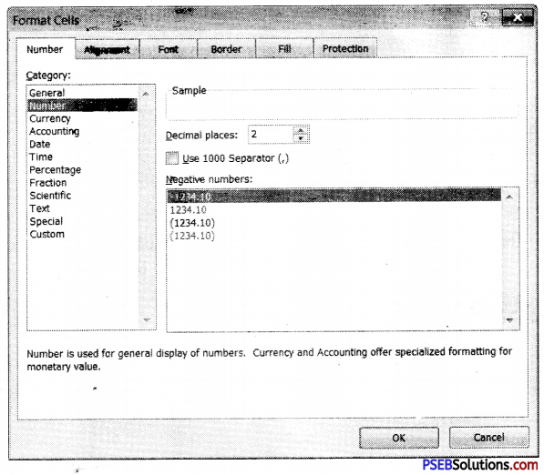
There are six tabs in the “Format Cells” window. All formatting options may be found on these tabs. Multiple cells can be formatted in one step by first selecting the cells and applying formatting.
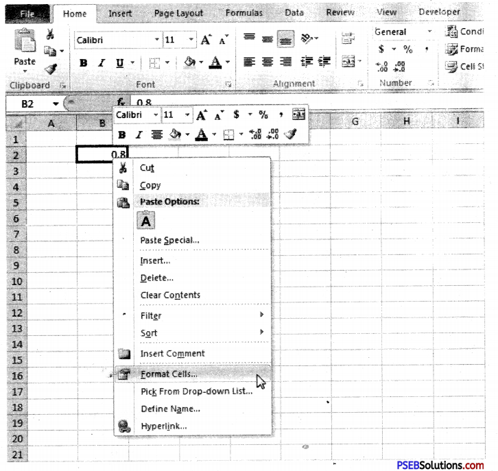
PSEB 9th Class Computer Notes Chapter 1 MS Excel Part-I 1 The “Format Cells” window can be opened in from the right-click menu. Formatting options are available on the Home Tab on the Font, Alignment, and Number groups.

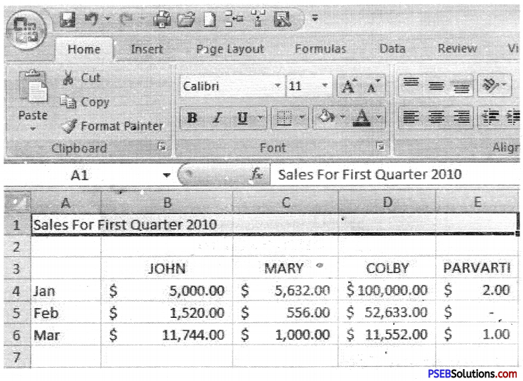
Merge and Centre

Merging cells is used when a text is to be centered over a particular section of a spreadsheet. When a group of cells is merged, then the text of this cell is merged as per selection and aligned center.
PSEB 9th Class Computer Notes Chapter 1 MS Excel Part-I 2
Following are the steps:

Type your data in your worksheet.
Highlight or select a range of cells.
Right-click on the highlighted cells and select Format Cells. Format Cells dialog box will open.
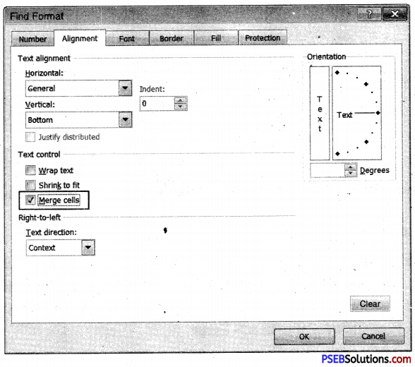
Click the Alignment tab of Format the checkbox labeled Merge cells as

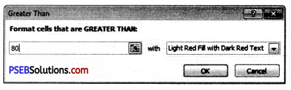
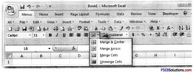
To merge a group of cells and center the text, we can also use the Merge and Center button on the Excel tool bar.
PSEB 9th Class Computer Notes Chapter 1 MS Excel Part-I 3

Steps:
1. Highlight or select a range of cells. Click the Merge and Center button on the toolbar.
Clicking this button will automatically merge our highlighted cells and center the cell value.
PSEB 9th Class Computer Notes Chapter 1 MS Excel Part-I 6

Numbers Group

A number format does not affect the actual cell value that Excel uses to perform calculations. The actual value is displayed in the formula bar. By applying different number formats, we can display numbers as percentages, dates, currency, and so on.

Number Formats available in MS Excel:

PSEB 9th Class Computer Notes Chapter 1 MS Excel Part-I 7

Styles in MS Excel:

A style is just a set of cell formatting settings. All cells to which a style has been applied look the same according to formatting. When we change a part of a style, all cells to which that style has been applied also change their formatting accordingly to new style.

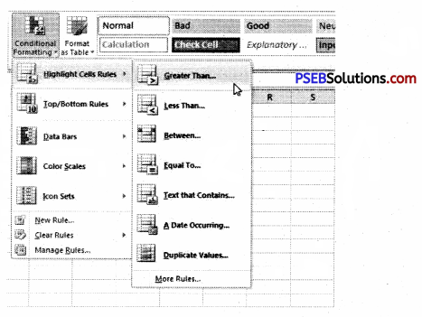
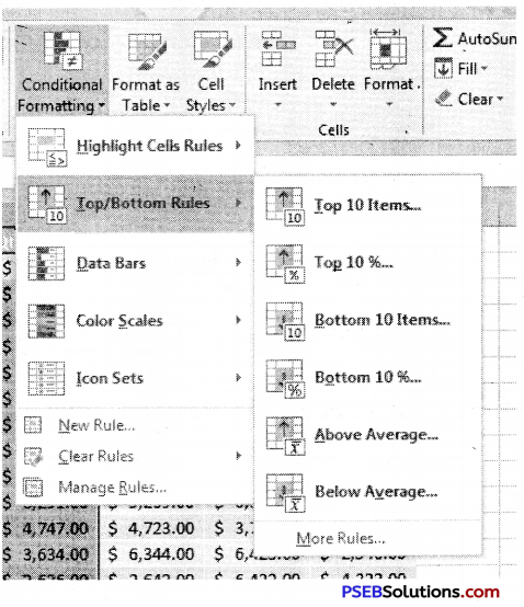
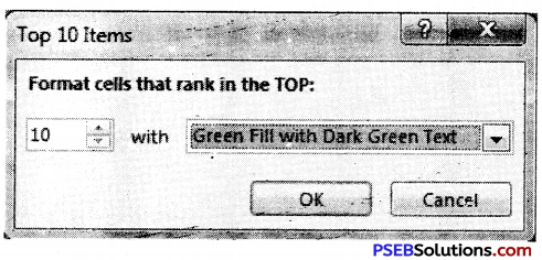
Conditional Formatting

Conditional Formatting is a tool in MS Excel that allows applying formats to a cell or range of cells. It also allows formatting change depending on the value of the cell or the value of a formula.

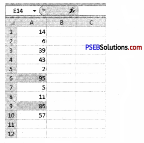
PSEB 9th Class Computer Notes Chapter 1 MS Excel Part-I 8

Formatting as Table

Tables can help to organize our content and make it easier for us to find the information we need.
To format information as a table:
PSEB 9th Class Computer Notes Chapter 1 MS Excel Part-I 9

1. Type the data in worksheet:

A	B	C	D	E
1. Code	Name	Colour	Unit Price	Unit Cost
2. ABC123	Widget	Red	10.15	7.18
3. ABC124	Widget	Green	10.9	6.981
4. ABC125	Widget	Blue	10.56	7.31
5. ABC 126	Gadget	Red	12.45	8.22
6. ABC 127	Gadget	Green	13.61	8.91

2. Select the cells we want to format as a table.
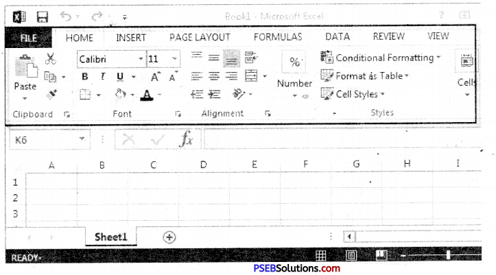
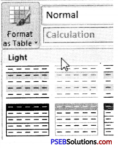
3. Click the Format as Table command in the Styles group on the Home tab.
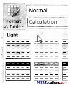
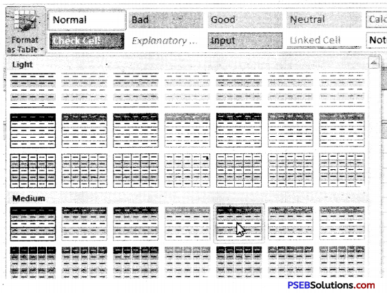
PSEB 9th Class Computer Notes Chapter 1 MS Excel Part-I 10
4. A list of predefined table styles will appear. Click a table style to select it.

5. A dialog box will appear confirming the range of cells we have selected for our table. The cells will appear selected in the spreadsheet and the range will appear in the dialog box.
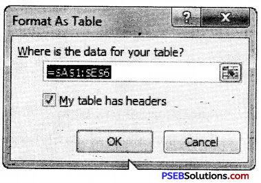
PSEB 9th Class Computer Notes Chapter 1 MS Excel Part-I 12
6. If necessary, change the range by selecting a new range of cells directly on your spreadsheet.
7. If our table has headers check the box next to My table has headers.
8. Click OK. The data will be formatted as a table.

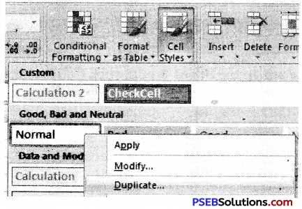
Cell Styles:

When we want to format cells in Microsoft Excel, we can do it manually either by selecting fonts, font color and size, background colors and borders, or we can do the formatting quickly and automatically using styles.

Microsoft Office Excel has several built-in cell styles that we can apply or modify. We can also modify or duplicate a cell style to create our own such as custom cell style.
PSEB 9th Class Computer Notes Chapter 1 MS Excel Part-I 13
Cell styles are based on the document theme that is applied to the whole workbook.

Applying a cell style:

1. Type the data in our worksheet
2. Select the cells that we want to format.
3. On the Home tab, in the Styles group, click Cell Styles.
PSEB 9th Class Computer Notes Chapter 1 MS Excel Part-I 14
Click the cell style that we want to apply. Our data will be changed according to our selected style.

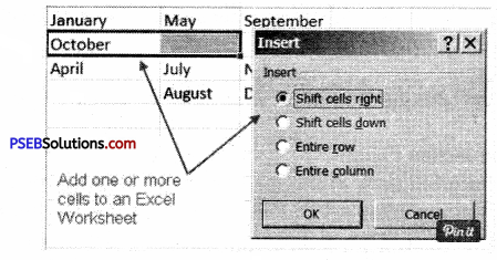
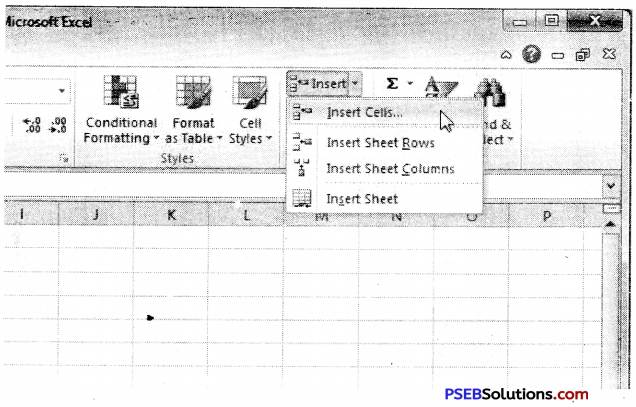
Cell Group:

To insert new cells, rows, or columns in an Excel worksheet, follow these steps:
1. Select the cells, rows, or columns where we want the new blank cells to appear.
2. Click the drop-down arrow attached to the Insert button in the Cells group of the Home tab.
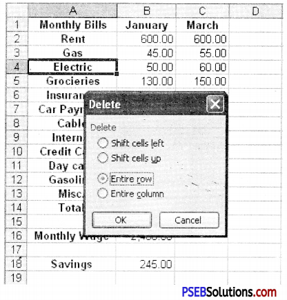
PSEB 9th Class Computer Notes Chapter 1 MS Excel Part-I 16
4. Click Delete Cells on the drop-down menu.

The Delete dialog box opens, showing these options for filling in the gaps:

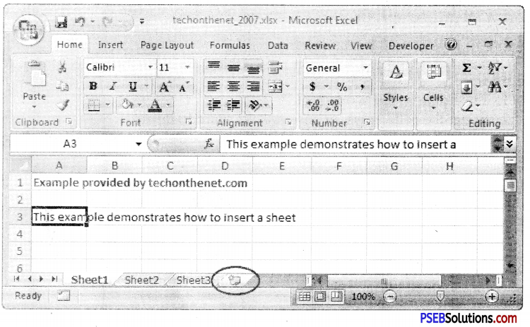
How to Insert New Worksheets?

As we can add new cells/row/columns in our existing worksheet, we can also add a new worksheet in our current workbook.
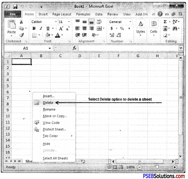
PSEB 9th Class Computer Notes Chapter 1 MS Excel Part-I 18

How To Delete Worksheets/worksheet?

A Single Worksheet or Worksheets can be deleted from a workbook, including those containing data.
1. Select the worksheet/worksheets we want to delete.
2. Right-click one of the selected worksheets. (The worksheet menu appears)
PSEB 9th Class Computer Notes Chapter 1 MS Excel Part-I 19
3. Select Delete. The selected worksheets will be deleted from our workbook.

Cell Size:

We can modify size of cells according to our requirement. We will learn how to change row height and column width.

How to modify column width?

1. Place our mouse over the column line in the column heading so the white cross becomes a double arrow.
2. Click and drag the column to the right to increase column width or to the left to decrease column width.
PSEB 9th Class Computer Notes Chapter 1 MS Excel Part-I 20
3. Release the mouse. The column width will be changed in your spreadsheet.

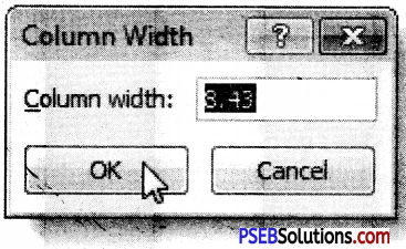
How to set column width with a specific measurement?

1. Select the columns we want to modify.
2. Click the Format command on the Home tab. The format drop-down menu appears.
PSEB 9th Class Computer Notes Chapter 1 MS Excel Part-I 21
3. Select Column Width.
4. The Column Width dialog box appears. Enter our specific measurement.

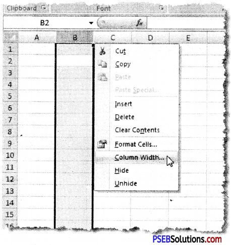
5. Click OK. The width of each selected column will be changed in our worksheet.

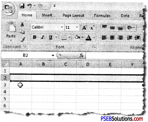
How to modify row height?

1. Place the cursor over the row line so the white cross becomes a double arrow.
2. Release the mouse. The height of each selected row will be changed in our worksheet.
PSEB 9th Class Computer Notes Chapter 1 MS Excel Part-I 23

How to set row height with a specific measurement?

1. Select the rows we want to modify.
2. Click the Format command on the Home tab. The format drop-down menu appears.
3. Select Row Height.
PSEB 9th Class Computer Notes Chapter 1 MS Excel Part-I 24
4. The Row Height dialog box appears. Enter a specific measurement.

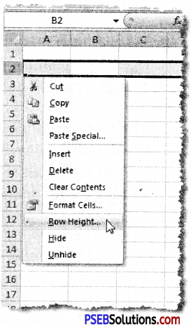
5. Click OK.

Formulas & Functions:

To maximize the capabilities of Excel, it is important to understand how to create simple formulas.
Creating simple formulas:
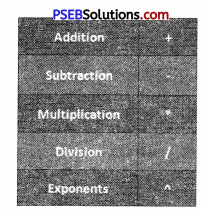
Excel uses standard operators for equations, such as a plus sign for addition (+), minus sign for subtraction (-), asterisk for multiplication (*), forward slash for division (/), and caret (A) for exponents. All formulas must begin with an equals sign (=).

To create a simple formula in Excel:
1. Select the cell where the answer will appear.
2. Type the equals sign (=).
3. Type in the formula we want Excel to calculate.
4. Press Enter. The formula will be calculated, and the value will be displayed in the cell.

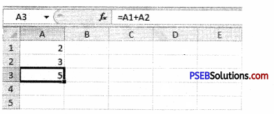
Creating formulas with cell references:

When a formula contains a cell address, it is called a cell reference. Creating a formula with cell references is useful because you can update data in our worksheet without having to rewrite the values in the formula.

To create a formula using cell references :

Select the cell where the answer will appear.
Type the equals sign (=).
Type the cell address that contains the first number in the equation.
Type the operator we need for our formula. For example, type the addition sign (+).
Type the cell address that contains the second number in the equation.
Press Enter. The formula will be calculated, and the value will be displayed in the cell.

Edit a Formula:

A formula in excel can be edited as per requirement.

Click the cell we want to edit.
Insert the cursor in the formula bar and edit the formula as desired. We can also double-click the cell to view and edit the formula directly from the cell or press F2 key.
When we’re done, press Enter or select the Enter command.

Cell Reference:

Cell Reference is termed to calculate important calculations by using a cell or a range of cells for a formula to calculate the result of the formula in a worksheet. We can use a cell reference for a single formula or for multiple formulas.

Types of Cell Reference

Relative Reference.
Absolute Reference.
Mixed Reference.

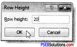
1. Relative Reference:

In Excel Relative reference is used by default. When it is copied to multiple cells then it changes according to cell position.
1. Type data in a worksheet.
2. Now type our formula in cell B1 = A1 * 10.
3. Drag the fill handle of cell Bl, we will see that the formula becomes in celi B2 = A2 * 10.
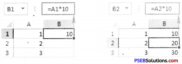
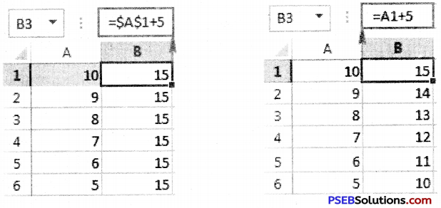
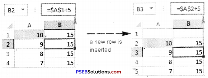
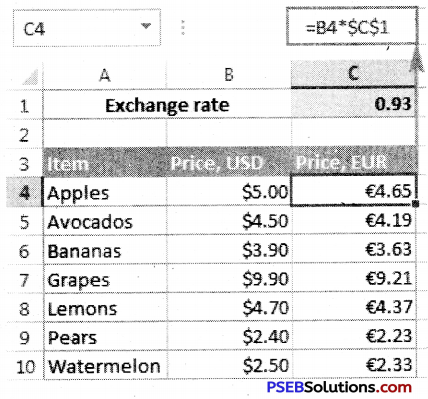
PSEB 9th Class Computer Notes Chapter 1 MS Excel Part-I 26

2. Absolute Reference:

Sometimes we want that during copying a formula from, one cell to another, its cell reference should not be changed. In this case Absolute Reference is used. Dollar($) sign is used during typing a formula using Absolute Reference. Dollar($) sign can be used either for a row or a column. We can also use it for both together.
PSEB 9th Class Computer Notes Chapter 1 MS Excel Part-I 27
1. Type data in a worksheet.
2. Now type our formula in cell B1=$A$1 + 5

3. Drag the fill handle of cell C1, we will see that the formula becomes in cell B2 = $A$1 + 5.

3. Mixed Reference:

Mixed Reference is the combination of both Relative and Absolute Reference. In Mixed Reference a Dollar($) sign is used either to a Row or Column.
PSEB 9th Class Computer Notes Chapter 1 MS Excel Part-I 30

Basic functions:

A function is a predefined formula that performs calculations using specific values in a particular order. They can save our time because we do not have to write the formula yourself. Excel has hundreds of functions to assist with our calculations.

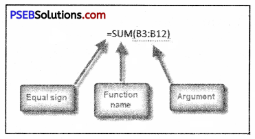
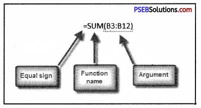
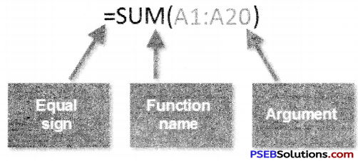
The parts of a function

The order in which we insert a function is important. Each function has a specific order – called syntax – which must be followed in order for the function to work correctly.
PSEB 9th Class Computer Notes Chapter 1 MS Excel Part-I 31
1. First of all equal to (=) sign is written.
2. After this the function name is written.
3. After this argument is written. Arguments contain the information we want the formula to calculate, such as a range of cell references.

Working with arguments:

Arguments are a vital-part of a Function.
1. Arguments must be enclosed in parentheses.
2. If there are Individual values or cell references inside the parentheses are separated by either colons or commas. Commas separate individual values, cell references, and cell ranges in parentheses.
PSEB 9th Class Computer Notes Chapter 1 MS Excel Part-I 32
3. If there is a ceil range in argument then it is written with colon in braces. Colons create a reference to a range of cells.

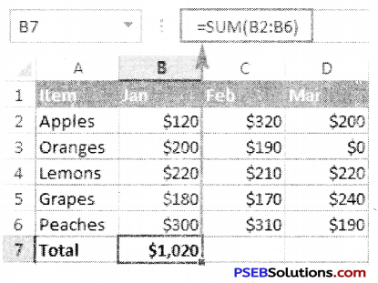
To create a basic function in Excel

1. Select the cell where the answer will appear (J3, for example).
2. Type the equals sign (=), then enter the function name (SUM, for example).
3. Enter the cells for the argument inside the parentheses.
4. Press Enter, and the result will appear.

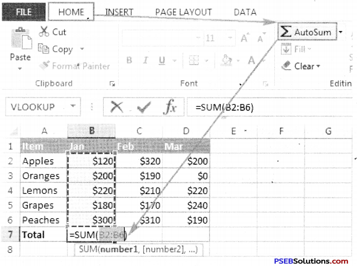
Using AutoSum to select common functions

The AutoSum command allows us to automatically return the results for a range of cells for common functions like SUM and AVERAGE.
1. Select the cell where the answer will appear.
2. Click the Home tab.
3. In the Editing group, click the AutoSum drop-down arrow and select the function we want.
PSEB 9th Class Computer Notes Chapter 1 MS Excel Part-I 33
4. A formula will appear the selected cell.
5. Press Enter, and the result will appear.

1. Text Functions:

Clean: This Function removes all non-printable characters from asupplied text string.
Trim: This Function removes duplicate spaces, and spaces at thestart and end of a text string
Concatenate: This Function Joins together two or more text strings
Left: This Function returns a specified number of characters fromthe start of a supplied text string
Mid: This Function Returns a specified numberfrom the middle of a supplied text string
Right: This Function Returns a specified numberfrom the end of a supplied text string

2. Logical Functions:

IF: This Function tests a user-defined condition and returns one result if the condition is TRUE, and another result if the condition is FALSE

3. Date and Time Functions:

Date: This Function returns a date, from a user-supplied year,month and day
Time: This Function returns a time, from a user-supplied hour, minute and second
Now: This Function returns the current date & time
Today: This Function returns today’s date

The Function Library:

To insert a function from the Function Library:
PSEB 9th Class Computer Notes Chapter 1 MS Excel Part-I 34
1. Type data in our worksheet.
2. Select the cell where the answer will appear.
3. Click the Formulas tab.
4. From the Function Library group, select the function category we want. In this example, we’ll choose Date & Time.

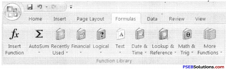
5. Select the desired function from the Date & Time drop-down menu
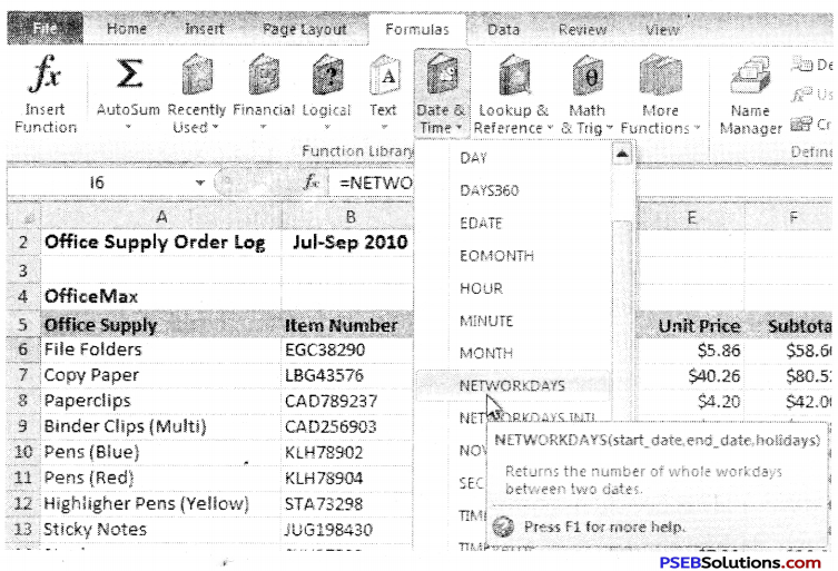
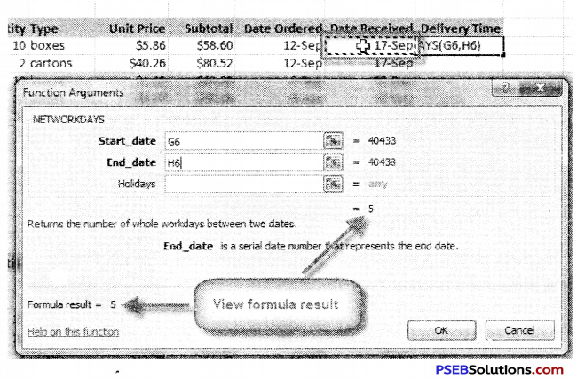
PSEB 9th Class Computer Notes Chapter 1 MS Excel Part-I 36
6. The Function Arguments dialog box will appear.

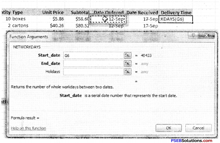
7. Click OK, and the result will appear.

Date Ordered	Date Received
12-Sep	17-Sep	5

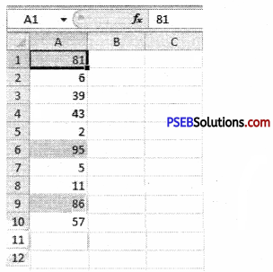
Sorting:

Sorting data in Excel basically means that we can arrange the data according to some specific criteria. We can even arrange data alphabetically:
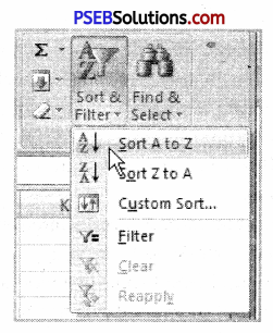
To sort in alphabetical order:
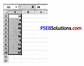
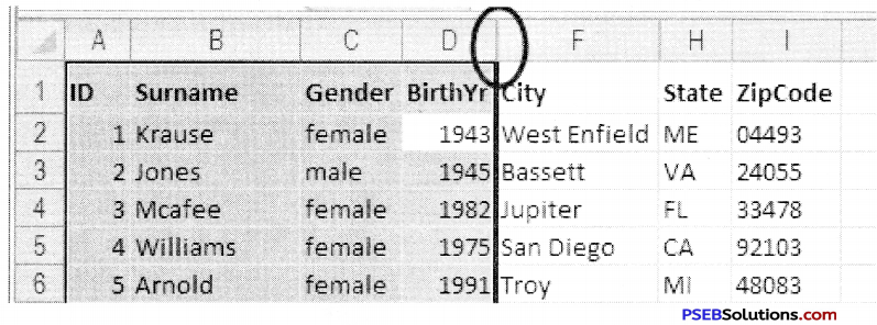
1. Type data in our worksheet.
2. Select a cell in the column we want to sort by.
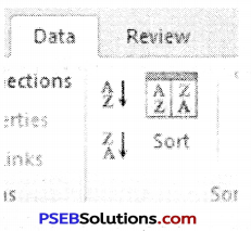
3. Select the Data tab, then locate the Sort and Filter group.
PSEB 9th Class Computer Notes Chapter 1 MS Excel Part-I 38
4. Click the ascending command to Sort A to Z or the descending command to Sort Z to A.

5. The data in the spreadsheet will be organized alphabetically.
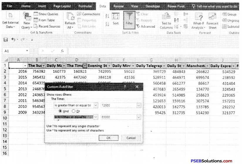
Filtering data: Filter is a tool in MS Excel that is used to get the information according to our requirement. When we need to find special information from a list, then we use Filter. Filters can be applied in different ways to improve the performance of our worksheet. We can filter text, dates, and numbers. We can even use more than one filter to further narrow our results.

Steps:

1. Type the data in a worksheet.
2. Select the Data tab, and then locate the Sort & Filter group.
3. Click the Filter command.
PSEB 9th Class Computer Notes Chapter 1 MS Excel Part-I 40
4. Drop-down arrows will appear in the header of each column.
5. Click the drop-down arrow for the column we want to filter.
6. The Filter menu appears.

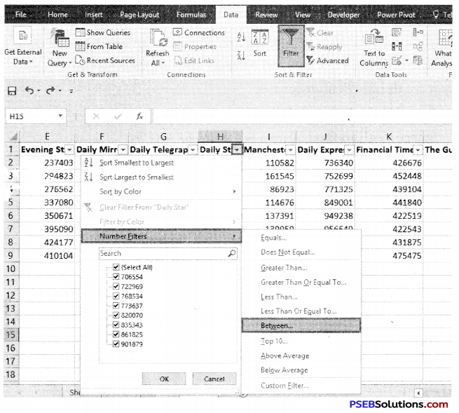
7. Uncheck the boxes next to the data we don’t want to view, or uncheck the box next to Select All to quickly uncheck all.
8. Check the boxes next to the data we do want to view.
9. Click OK.
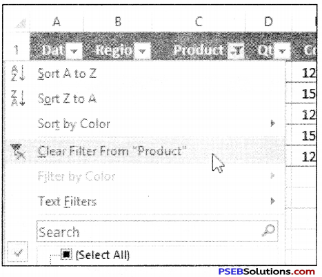
To clear a filter: We can clear a filter very easily.
1. Click the drop-down arrow in the column from which we want to clear the filter.
2. Choose Clear Filter From.
PSEB 9th Class Computer Notes Chapter 1 MS Excel Part-I 42
3. The filter will be cleared from the column. The data that was previously hidden will be on display once again.

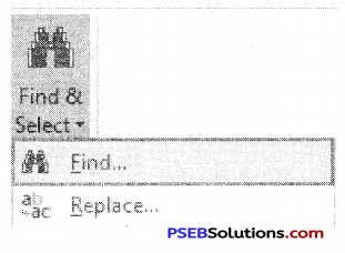
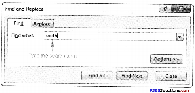
Find and Replace

Excel Find and Replace feature are powerful tools that we can use for special criteria such as to Find a text and to Replace it with our new text.

How to use Find Option:

Following are the steps to locate data in a worksheet:
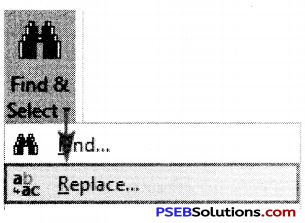
1. Choose Find & Select in the Editing group on the Home tab, and then select Find (or press Ctrl+F).The Find and Replace dialog box appears with the Find tab on top.
PSEB 9th Class Computer Notes Chapter 1 MS Excel Part-I 43
2. In the Find What box, enter the data we want to locate.

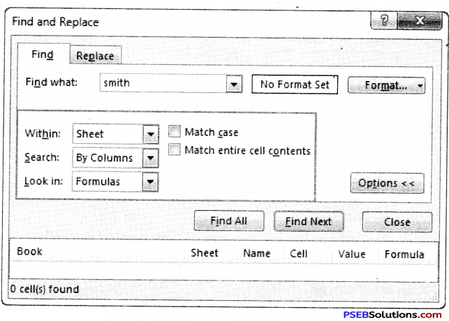
3. Click the Options button to expand the dialog box.
1. Within: It searches just the current worksheet or the entire workbook.
2. Search: It selects whether to search first across the rows or down the columns.
3. Look In: It selects whether we want to search through the values or formula results, through the actual formulas, or if we want to look in the comments.
4. Match Case: It checks this box if we want our search to be case-specific.
List only the items that exactly match our search criteria.
PSEB 9th Class Computer Notes Chapter 1 MS Excel Part-I 45
3. Click Find Next.
Excel jumps to the first occurrence of the match.
4. Click Close when we’ve located the entry we want.
Using Replacing data Option: Replace option is used to change data according to our requirement. We can change each entry of a cell while typing on, but it require more time and labour so we can do it easily using Replace option.
1. Choose Find & Select in the Editing group on the Home tab, and then select Replace (or press Ctrl+H).The Find and Replace dialog box appears with the Replace tab on top.
PSEB 9th Class Computer Notes Chapter 1 MS Excel Part-I 46
2. In the Find What box, enter the data we want to locate.

3. In the Replace With box, enter the data with which we want to replace the found data.
4. Click the Options button and specify any desired options.

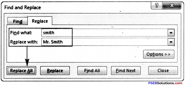
Click Find Next to locate the first occurrence or click Find All to display a list of all occurrences.
Click OK in the alert box and then click Close.

PSEB 9th Class Computer Solutions Chapter 1 MS Excel Part-I

November 2, 2021November 1, 2021 by Prasanna

Punjab State Board PSEB 9th Class Computer Book Solutions Chapter 1 MS Excel Part-I Textbook Exercise Questions and Answers.

PSEB Solutions for Class 9 Computer Science Chapter 1 MS Excel Part-I

Computer Guide for Class 9 PSEB MS Excel Part-I Textbook Questions and Answers

1. Fill in the Blanks

1. An Excel Workbook consists of ………………………
(a) Worksheets
(b) Rows
(c) Columns
(d) Formulas
Answer:
Worksheets

2. The actual value of a cell is displayed in …………………….. bar.
(a) Title
(b) Menu
(c) Formula
(d) None of these
Answer:
Formula

3. …………………….. Formatting applies one or more rules to any cells you want.
(a) Formula
(b) Function
(c) Conditional
(d) None of these
Answer:
Conditional

4. Format Command is available on ………………… Tab.
(a) Home
(b) Insert
(c) Data
(d) Formulas
Answer:
Home

5. All Formulas must begin with an ………………………… sign.
(a) Sigma
(b) Plus
(c) Equal
(d) None of these
Answer:
Equal

6. A data in your worksheet can be arranged in an order using ………………………
(a) Formula
(b) Function
(c) Filter
(d) Sorting
Answer:
Sorting

7. Sort & Filter command is available on ……………………Tab.
(a) Home
(b) Insert
(c) Data
(d) Formulas
Answer:
Data

2. Short Answer Type Questions

Question 1.
What is Formatting?
Answer:
Formats are changes that are made to Excel worksheets in order to enhance their appearance and/or to focus attention on specific data in the worksheet. Formatting changes the appearance of data but does not change the actual data in the cell, which can be important if that data is used in calculations. For example, formatting numbers to display only two decimal places does not shorten or round values with more than two decimal places. To actually alter the numbers in this way, the data would need to be rounded using one of Excel’s rounding functions.

Question 2.
Define Number Format in Excel.
Answer:
By applying different number formats, you can change the appearance of a number without changing the number itself. A number format does not affect the actual cell value that Excel uses to perform calculations. The actual value is displayed in the formula bar. By applying different number formats, you can display numbers as percentages, dates, currency, and so on.

Question 3.
What are the standard operators used in simple formulas?
Answer:
Excel uses standard operators for formulas, such as a plus sign for addition (+), a minus sign for subtraction (-), an asterisk for multiplication (*), a forward slash for division (/), and a caret (Λ) for exponents.
PSEB 9th Class Computer Solutions Chapter 1 MS Excel Part-I Img 1
All formulas in Excel must begin with an equals sign (=). This is because the cell contains, or is equal to, the formula and the value it calculates.

Question 4.
What is a cell reference?
Answer:
A cell reference refers to a cell or a range of cells on a worksheet and can be used in a formula so that Microsoft Office Excel can find the values or data that you want that formula to calculate.
In one or several formulas, you can use a cell reference to refer to :

Data from one cell on the worksheet.
Data is contained in different areas of a worksheet.
Data in cells on other worksheets in the same workbook.

Question 5.
What are the parts of a Function?
Answer:
The order in which you insert a function is important. Each function has a specific order—called syntax — which must be followed in order for the function to work correctly. The basic syntax to create a formula with a function is to insert an equals sign (=), function name (SUM, for example, is the function name for addition), and argument. Arguments contain the information you want the formula to calculate, such as a range of cell references.
PSEB 9th Class Computer Solutions Chapter 1 MS Excel Part-I Img 2

Question 6.
Define Sorting.
Answer:
Sorting is a common spreadsheet task that allows you to easily reorder your data. The most common type of sorting is alphabetical ordering, which you can do in ascending or descending order.
To sort in alphabetical order :

Select a cell in the column you want to sort (In this example, we choose a cell in column A).
Click the Sort & Filter command in the Editing group on the Home tab.
Select Sort A fo Z. NOWT the information in the Category column is organized in alphabetical order.

PSEB 9th Class Computer Solutions Chapter 1 MS Excel Part-I Img 3

You can sort in reverse alphabetical order by choosing Sort Z to A in the list.

Question 7.
Define Filter.
Answer:
The basic Excel filter (also known as the Excel Autofilter) allows you to view specific rows in an Excel spreadsheet while hiding the other rows in the worksheet. When a filter is added to the header row of a spreadsheet, a drop-down menu appears on each cell of the header row. This provides you with a number of filter options that can be used to specify which rows of the spreadsheet are to be displayed.

3. Long Answer Type Questions

Question 1.
What are Merge and Centre? Write down the steps to merge a group of cells.
Answer:
If you go to the Home menu in the ribbon and look in the Alignment grouping of commands, you will see a small icon in the lower, right-hand corner called Merge and Center. This command does just what it implies. It not only merges the cells into one larger cell, but it also centers the text. Merge and Center improves the appearance of a title or header by centering the text over a particular section of the spreadsheet. If you click on the More icon to the Merge and Center command, you will see other Merge options.

The first one is Merge Across. This will merge multiple cells and more than one row at the same time. The text will remain left-justified.
Then there are Merge Cells. This will merge multiple cells on one row and will keep the text left-justified.
Finally, you have Unmerge Cells, which will undo the merged cells.

Let’s take a look at an example using the Merge and Center command. Imagine you are a painting contractor for residential homes. You created a spreadsheet to include several different costs for work requested by a new client. You have everything formatted nicely. The title, which includes the name of the client, the estimated number, and street address has been entered into cell Al. It would be nice if we could quickly and easily center the title across the top of the spreadsheet. Here are the steps.

Highlight the cells you want to merge. (In our example, Al through FI),
Go to the Home menu in the ribbon.
Look in the Alignment grouping of commands.
Click on Merge and Center.

Just like that, your title is centered and the cells have been merged into one larger cell. The benefit? Well, besides it looks better, you can make changes to the cells below and the title will remain centered: For instance, you can add a column (or delete one) and your title will not be affected. One important note about the Merge command: merging cells can delete data. Only the data in the upper-left cell will be kept once the cells have merged. Do not place data in every cell if you plan on merging multiple cells into one larger cell.

Question 2.
What is Conditional Formatting? Write down the steps to create a conditional formatting rule.
Answer:
Conditional formatting in Excel enables you to highlight cells with a certain color, depending on the cell’s value.
Highlight Cells Rules
To highlight cells that are greater than a value, execute the following steps.
1. Select the range A1:A10.
PSEB 9th Class Computer Solutions Chapter 1 MS Excel Part-I Img 4

2. On the Home tab, click Conditional Formatting, Highlight Cells Rules, Greater Than…
PSEB 9th Class Computer Solutions Chapter 1 MS Excel Part-I Img 5

3. Enter the value 80 and select a formatting style.
PSEB 9th Class Computer Solutions Chapter 1 MS Excel Part-I Img 6

4. Click OK.
Result. Excel highlights the cells that are greater than 80.
PSEB 9th Class Computer Solutions Chapter 1 MS Excel Part-I Img 7

5. Change the value of cell A1 to 81.
Result. Excel changes the format of cell A1 automatically.
PSEB 9th Class Computer Solutions Chapter 1 MS Excel Part-I Img 8

Question 3.
What is a cell? How can we insert a new cell in our current worksheet?
Answer:
A cell is an intersection between a row and a column on a spreadsheet that starts with cell Al. Below is an illustrated example of a highlighted cell in Microsoft Excel; the cell address, cell name, or cell pointer “D8” (column D, row 8) is the selected cell and the location of what is being modified.
Insert Cells into an Excel Worksheet
Having to insert extra cells to an Excel worksheet from time to time is a common practice: data gets forgotten and must be added, space must be made for new data, or existing data gets moved about when the sheet is reorganized.
Whatever the reason, there is, as is the case with all Microsoft programs, more than one way to accomplish the task of inserting cells to an Excel worksheet.
PSEB 9th Class Computer Solutions Chapter 1 MS Excel Part-I Img 9

Question 4.
What is a Formula? Write down the steps to create a simple Formula in Excel.
Answer:
A formula is an expression that calculates the value of a cell. Functions are predefined formulas and are already available in Excel. For example, cell A3 below contains a formula that adds the value of cell A2 to the value of cell A1.
PSEB 9th Class Computer Solutions Chapter 1 MS Excel Part-I Img 10

Steps to create a simple formula in MS Excel
You can create a simple formula to add, subtract, multiply or divide values in your worksheet. Simple formulas always start with an equal sign (=), followed by constants that are numeric values and calculation operators such as plus (+), minus (-), an asterisk(*), or forward-slash (/) signs.
For example, when you enter the formula =5+2*3, Excel multiplies the last two numbers and adds the first number to the result. Following the standard order of mathematical operations, multiplication is performed before addition.

On the worksheet, click the cell in which you want to enter the formula.
Type the = (equal sign) followed by the constants and operators that you want to use in the calculation.

You can enter as many constants and operators in a formula as you need, up to 8192 characters.

Question 5.
What is a Function? Write down the steps to create a basic Function in Excel.
Answer:
In Excel, a function is a preset formula used for calculations. Like formulas, functions begin with the equal sign ( = ) followed by the function’s name and its arguments. The function name tells Excel what calculation to perform. The arguments are contained inside round brackets. For example, the most used function in Excel is the function, which is used to add together the data in selected cells.

The SUM function is written as –
= SUM (D1: D6 )
Here the function adds the contents of cell range D1 to D6 and displays the answer in cell D7.

The parts of a function :
The order in which you insert a function is important. Each function has a specific order called syntax—which must be followed in order for the function to work correctly. The basic syntax to create a formula with a function is to insert an equals sign (=), function name (SUM, for example, is the function name for addition), and argument. Arguments contain the information you want the formula to calculate, such as a range of cell references.
PSEB 9th Class Computer Solutions Chapter 1 MS Excel Part-I Img 11

PSEB 9th Class Computer Guide MS Excel Part-I Important Questions and Answers

Fill in the Blanks

1. Format Cell window contains …………………… Labs.
(a) 5
(b) 6
(c) 7
(d) 8
Answer:
(b) 6

2. Excel has ……………………. Number formats.
(a) 6
(b) 8
(c) 10
(d) 12
Answer:
(d) 12

3. Insert/Delete dialog box has ………………. options.
(a) 4
(b) 5
(c) 6
(d) 7
Answer:
(a) 4

4. Workbook contains sheets by default.
(a) 2
(b) 3
(c) 4
(d) 5
Answer:
(b) 3

5. Arranged data in ascending or descending order is called …………………
(a) Formatting
(b) Splitting
(c) Sorting
(d) Replacing
Answer:
(c) Sorting

6. Cell address used in the formula is called ……………………………………..
(a) Function
(b) Formula
(c) Address
(d) Reference
Answer:
(d) Reference

Short Answer Type Questions

Question 1.
What is Microsoft Excel?
Answer:
Microsoft Excel is an electronic worksheet developed by Microsoft, to be used for organizing, storing, and manipulating.

Question 2.
What is a ribbon?
Answer:
The ribbon runs on the top of the application and is the replacement for the toolbars and menus. The ribbons have various tabs on the top, and each tab has its own group of commands.

Question 3.
How can I hide or show the ribbon?
Answer:
Use the CTRL and FI key to toggle & show or hide the ribbon.

Question 4.
How can you wrap the text within a cell?
Answer:
You have to select the text you want to wrap, and then click wrap text from the home tab and you can wrap the text within a cell.
PSEB 9th Class Computer Solutions Chapter 1 MS Excel Part-I Img 12

Question 5.
Is it possible to prevent someone from copying the cell from your worksheet?
Answer:
Yes, it is possible. In order to protect your worksheet from getting copied, you need to go into Menu bar >Review > Protect sheet > Password. By entering the password, you can secure your worksheet from getting copied by others.

Question 6.
How you can sum up the Roi4p and Column number quickly in the excel sheet?
Answer:
By using the SUM function you can get the total sum of the rows arid columns, in an excel worksheet.

Question 7.
How you can add a new excel worksheet?
Answer:
To add a new Excel worksheet you have to insert a worksheet tab at the bottom of the screen.

Question 8.
How you can resize the column?
Answer:
To resize the column you have to change the width of one column and then drag the boundary on the right side of the column heading to the width you want. The other way of doing it is to select the Format from the home tab, and in Format, you have to select AUTOFIT COLUMN WIDTH under the cell section. On clicking on this the cell size will get formatted.

Question 9.
What are three report formats that are available in Excel?
Answer:
The three report formats in Excel are :

Compact
Report
Tabular

Question 10.
How would, you provide a Dynamic range in the “Data Source” of Pivot Tables?
Answer:
To provide a dynamic range in the “Data Source” of Pivot tables, first, create a named range using offset function and base the pivot table using a named range created in the first step.

Question 11.
Is it possible to make a Pivot table using multiple sources of data?
Answer:
If the multiple sources are different worksheets, from the same workbook/then it is possible to make a Pivot table using multiple sources of data.

Long Answer Type Questions

Question 1.
How do you create formulas in Excel?
Answer:
Create a simple formula in Excel with constants and calculation operators.
To create a simple calculation, click the cell in which you wish to enter the formula and type an equal sign. Enter the constants and operators that you wish to use in the calculation within the cell. Use the plus sign for addition, a minus sign for subtraction, the backslash for division, and the asterisk for multiplication. For instance, to add ten and ten in a cell, enter “=10+10” within the desired cell and press the Enter key.

Question 2.
Write the various steps for inserting a single cell into a worksheet.
Ans. The first example will insert a single cell to column A in order to make room for the month of March. To do this April will be shifted downward to cell A4.

Click on cell A3 to make it the active cell
Right-click on cell A3 to open the right-click menu
Click on Insert in the right-click menu to open the Insert cells dialog box
Click on the Shift cells down option in the dialog box
Click OK to add the one cell to the worksheet and to close the dialog box
Cell A3 should now be blank and April should be located in cell A4
Type March into cell A3

Question 3.
Write the various steps for inserting multiple cells into a worksheet.
Answer:
The second example will insert two additional cells to row two in order to make room for February and June in cells A2 and B2. In the process, October will be shifted to cell C3.

Drag select cells A2 and B2 in the worksheet to highlight them
Right-click on cells B2 to open the right-click menu
Click on Insert in the right-click menu to open the Insert cells dialog box
Click on the Shift cells right option in the dialog box
Click OK to add the two cells to the worksheet and to close the dialog box
Cells A2 and B2 should now be blank and October should be located in cell C3
Type February into cell A2 and June into cell B2.

Question 4.
Discuss the cell reference in Excel.
Answer:
For many spreadsheets, you won’t want to go back to the original formula to change all the information you’re working with. This is where cell references come in handy. By entering a reference to another cell on the worksheet, you can tell the formula to work its calculation with whatever number is placed in that cell. The formula can then be changed quickly by trying out different numbers in the reference cell.

To reference a cell, simply enter the location of the call as designated by its column and row; for example, A1 is the cell in the top left corner of the spreadsheet. To reference a cell on another worksheet within the same workbook, type the name of the worksheet followed by an exclamation point, then the location of the cell. So Sheet !A1 would refer to the A1 cell on the worksheet titled “Sheet.” If you want to reference a range of cells, use a colon between the first and last cell of the range. The formula =SUM(A1:A12) will calculate the total sum of all the figures in the range from A1 down to A12.

Question 5.
Demonstrate the use of AutoSum in Excel.
Answer:
Using AutoSum to select common functions
The AutoSum command allows you to automatically return the results for a range of cells for common functions like SUM and AVERAGE.

Select the cell where the answer will appear (E24, for example).
Click the Home tab.
In the Editing group, click the AutoSum drop-down arrow and select the function you want (Average, for example).