MS Excel Part-I Notes

Punjab State Board PSEB 9th Class Computer Book Solutions Chapter 1 MS Excel Part-I Textbook Exercise Questions and Answers.

PSEB Solutions for Class 9 Computer Science Chapter 1 MS Excel Part-I

Computer Guide for Class 9 PSEB MS Excel Part-I Textbook Questions and Answers

1. Fill in the Blanks

1. An Excel Workbook consists of ………………………
(a) Worksheets
(b) Rows
(c) Columns
(d) Formulas
Answer:
Worksheets

2. The actual value of a cell is displayed in …………………….. bar.
(a) Title
(b) Menu
(c) Formula
(d) None of these
Answer:
Formula

3. …………………….. Formatting applies one or more rules to any cells you want.
(a) Formula
(b) Function
(c) Conditional
(d) None of these
Answer:
Conditional

4. Format Command is available on ………………… Tab.
(a) Home
(b) Insert
(c) Data
(d) Formulas
Answer:
Home

5. All Formulas must begin with an ………………………… sign.
(a) Sigma
(b) Plus
(c) Equal
(d) None of these
Answer:
Equal

6. A data in your worksheet can be arranged in an order using ………………………
(a) Formula
(b) Function
(c) Filter
(d) Sorting
Answer:
Sorting

7. Sort & Filter command is available on ……………………Tab.
(a) Home
(b) Insert
(c) Data
(d) Formulas
Answer:
Data

2. Short Answer Type Questions

Question 1.
What is Formatting?
Answer:
Formats are changes that are made to Excel worksheets in order to enhance their appearance and/or to focus attention on specific data in the worksheet. Formatting changes the appearance of data but does not change the actual data in the cell, which can be important if that data is used in calculations. For example, formatting numbers to display only two decimal places does not shorten or round values with more than two decimal places. To actually alter the numbers in this way, the data would need to be rounded using one of Excel’s rounding functions.

Question 2.
Define Number Format in Excel.
Answer:
By applying different number formats, you can change the appearance of a number without changing the number itself. A number format does not affect the actual cell value that Excel uses to perform calculations. The actual value is displayed in the formula bar. By applying different number formats, you can display numbers as percentages, dates, currency, and so on.

Question 3.
What are the standard operators used in simple formulas?
Answer:
Excel uses standard operators for formulas, such as a plus sign for addition (+), a minus sign for subtraction (-), an asterisk for multiplication (*), a forward slash for division (/), and a caret (Λ) for exponents.

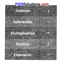
All formulas in Excel must begin with an equals sign (=). This is because the cell contains, or is equal to, the formula and the value it calculates.

Question 4.
What is a cell reference?
Answer:
A cell reference refers to a cell or a range of cells on a worksheet and can be used in a formula so that Microsoft Office Excel can find the values or data that you want that formula to calculate.
In one or several formulas, you can use a cell reference to refer to :

• Data from one cell on the worksheet.
• Data is contained in different areas of a worksheet.
• Data in cells on other worksheets in the same workbook.

Question 5.
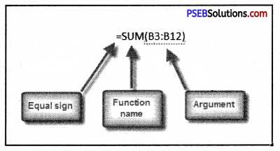
What are the parts of a Function?
Answer:
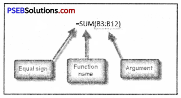
The order in which you insert a function is important. Each function has a specific order—called syntax — which must be followed in order for the function to work correctly. The basic syntax to create a formula with a function is to insert an equals sign (=), function name (SUM, for example, is the function name for addition), and argument. Arguments contain the information you want the formula to calculate, such as a range of cell references.

Question 6.
Define Sorting.
Answer:
Sorting is a common spreadsheet task that allows you to easily reorder your data. The most common type of sorting is alphabetical ordering, which you can do in ascending or descending order.
To sort in alphabetical order :

• Select a cell in the column you want to sort (In this example, we choose a cell in column A).
• Click the Sort & Filter command in the Editing group on the Home tab.
• Select Sort A fo Z. NOWT the information in the Category column is organized in alphabetical order.

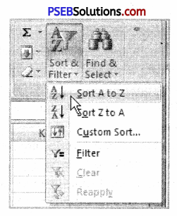
You can sort in reverse alphabetical order by choosing Sort Z to A in the list.

Question 7.
Define Filter.
Answer:
The basic Excel filter (also known as the Excel Autofilter) allows you to view specific rows in an Excel spreadsheet while hiding the other rows in the worksheet. When a filter is added to the header row of a spreadsheet, a drop-down menu appears on each cell of the header row. This provides you with a number of filter options that can be used to specify which rows of the spreadsheet are to be displayed.

3. Long Answer Type Questions

Question 1.
What are Merge and Centre? Write down the steps to merge a group of cells.
Answer:
If you go to the Home menu in the ribbon and look in the Alignment grouping of commands, you will see a small icon in the lower, right-hand corner called Merge and Center. This command does just what it implies. It not only merges the cells into one larger cell, but it also centers the text. Merge and Center improves the appearance of a title or header by centering the text over a particular section of the spreadsheet. If you click on the More icon to the Merge and Center command, you will see other Merge options.

• The first one is Merge Across. This will merge multiple cells and more than one row at the same time. The text will remain left-justified.
• Then there are Merge Cells. This will merge multiple cells on one row and will keep the text left-justified.
• Finally, you have Unmerge Cells, which will undo the merged cells.

Let’s take a look at an example using the Merge and Center command. Imagine you are a painting contractor for residential homes. You created a spreadsheet to include several different costs for work requested by a new client. You have everything formatted nicely. The title, which includes the name of the client, the estimated number, and street address has been entered into cell Al. It would be nice if we could quickly and easily center the title across the top of the spreadsheet. Here are the steps.

1. Highlight the cells you want to merge. (In our example, Al through FI),
2. Go to the Home menu in the ribbon.
3. Look in the Alignment grouping of commands.
4. Click on Merge and Center.

Just like that, your title is centered and the cells have been merged into one larger cell. The benefit? Well, besides it looks better, you can make changes to the cells below and the title will remain centered: For instance, you can add a column (or delete one) and your title will not be affected. One important note about the Merge command: merging cells can delete data. Only the data in the upper-left cell will be kept once the cells have merged. Do not place data in every cell if you plan on merging multiple cells into one larger cell.

Question 2.
What is Conditional Formatting? Write down the steps to create a conditional formatting rule.
Answer:
Conditional formatting in Excel enables you to highlight cells with a certain color, depending on the cell’s value.
Highlight Cells Rules
To highlight cells that are greater than a value, execute the following steps.
1. Select the range A1:A10.

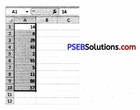
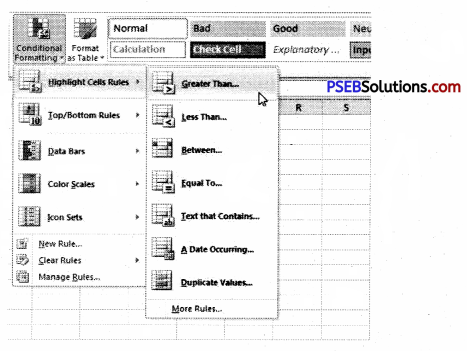
2. On the Home tab, click Conditional Formatting, Highlight Cells Rules, Greater Than…

3. Enter the value 80 and select a formatting style.

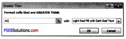
4. Click OK.
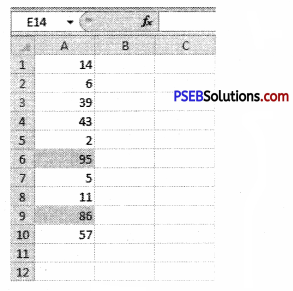
Result. Excel highlights the cells that are greater than 80.

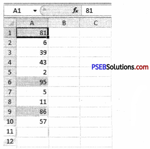
5. Change the value of cell A1 to 81.
Result. Excel changes the format of cell A1 automatically.

Question 3.
What is a cell? How can we insert a new cell in our current worksheet?
Answer:
A cell is an intersection between a row and a column on a spreadsheet that starts with cell Al. Below is an illustrated example of a highlighted cell in Microsoft Excel; the cell address, cell name, or cell pointer “D8” (column D, row 8) is the selected cell and the location of what is being modified.
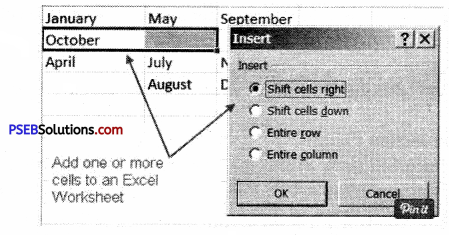
Insert Cells into an Excel Worksheet
Having to insert extra cells to an Excel worksheet from time to time is a common practice: data gets forgotten and must be added, space must be made for new data, or existing data gets moved about when the sheet is reorganized.
Whatever the reason, there is, as is the case with all Microsoft programs, more than one way to accomplish the task of inserting cells to an Excel worksheet.

Question 4.
What is a Formula? Write down the steps to create a simple Formula in Excel.
Answer:
A formula is an expression that calculates the value of a cell. Functions are predefined formulas and are already available in Excel. For example, cell A3 below contains a formula that adds the value of cell A2 to the value of cell A1.

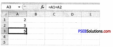
Steps to create a simple formula in MS Excel
You can create a simple formula to add, subtract, multiply or divide values in your worksheet. Simple formulas always start with an equal sign (=), followed by constants that are numeric values and calculation operators such as plus (+), minus (-), an asterisk(*), or forward-slash (/) signs.
For example, when you enter the formula =5+2*3, Excel multiplies the last two numbers and adds the first number to the result. Following the standard order of mathematical operations, multiplication is performed before addition.

1. On the worksheet, click the cell in which you want to enter the formula.
2. Type the = (equal sign) followed by the constants and operators that you want to use in the calculation.

You can enter as many constants and operators in a formula as you need, up to 8192 characters.

Question 5.
What is a Function? Write down the steps to create a basic Function in Excel.
Answer:
In Excel, a function is a preset formula used for calculations. Like formulas, functions begin with the equal sign ( = ) followed by the function’s name and its arguments. The function name tells Excel what calculation to perform. The arguments are contained inside round brackets. For example, the most used function in Excel is the function, which is used to add together the data in selected cells.

The SUM function is written as –
= SUM (D1: D6 )
Here the function adds the contents of cell range D1 to D6 and displays the answer in cell D7.

The parts of a function :
The order in which you insert a function is important. Each function has a specific order called syntax—which must be followed in order for the function to work correctly. The basic syntax to create a formula with a function is to insert an equals sign (=), function name (SUM, for example, is the function name for addition), and argument. Arguments contain the information you want the formula to calculate, such as a range of cell references.

PSEB 9th Class Computer Guide MS Excel Part-I Important Questions and Answers

Fill in the Blanks

1. Format Cell window contains …………………… Labs.
(a) 5
(b) 6
(c) 7
(d) 8
Answer:
(b) 6

2. Excel has ……………………. Number formats.
(a) 6
(b) 8
(c) 10
(d) 12
Answer:
(d) 12

3. Insert/Delete dialog box has ………………. options.
(a) 4
(b) 5
(c) 6
(d) 7
Answer:
(a) 4

4. Workbook contains sheets by default.
(a) 2
(b) 3
(c) 4
(d) 5
Answer:
(b) 3

5. Arranged data in ascending or descending order is called …………………
(a) Formatting
(b) Splitting
(c) Sorting
(d) Replacing
Answer:
(c) Sorting

6. Cell address used in the formula is called ……………………………………..
(a) Function
(b) Formula
(c) Address
(d) Reference
Answer:
(d) Reference

Short Answer Type Questions

Question 1.
What is Microsoft Excel?
Answer:
Microsoft Excel is an electronic worksheet developed by Microsoft, to be used for organizing, storing, and manipulating.

Question 2.
What is a ribbon?
Answer:
The ribbon runs on the top of the application and is the replacement for the toolbars and menus. The ribbons have various tabs on the top, and each tab has its own group of commands.

Question 3.
How can I hide or show the ribbon?
Answer:
Use the CTRL and FI key to toggle & show or hide the ribbon.

Question 4.
How can you wrap the text within a cell?
Answer:
You have to select the text you want to wrap, and then click wrap text from the home tab and you can wrap the text within a cell.

Question 5.
Is it possible to prevent someone from copying the cell from your worksheet?
Answer:
Yes, it is possible. In order to protect your worksheet from getting copied, you need to go into Menu bar >Review > Protect sheet > Password. By entering the password, you can secure your worksheet from getting copied by others.

Question 6.
How you can sum up the Roi4p and Column number quickly in the excel sheet?
Answer:
By using the SUM function you can get the total sum of the rows arid columns, in an excel worksheet.

Question 7.
How you can add a new excel worksheet?
Answer:
To add a new Excel worksheet you have to insert a worksheet tab at the bottom of the screen.

Question 8.
How you can resize the column?
Answer:
To resize the column you have to change the width of one column and then drag the boundary on the right side of the column heading to the width you want. The other way of doing it is to select the Format from the home tab, and in Format, you have to select AUTOFIT COLUMN WIDTH under the cell section. On clicking on this the cell size will get formatted.

Question 9.
What are three report formats that are available in Excel?
Answer:
The three report formats in Excel are :

• Compact
• Report
• Tabular

Question 10.
How would, you provide a Dynamic range in the “Data Source” of Pivot Tables?
Answer:
To provide a dynamic range in the “Data Source” of Pivot tables, first, create a named range using offset function and base the pivot table using a named range created in the first step.

Question 11.
Is it possible to make a Pivot table using multiple sources of data?
Answer:
If the multiple sources are different worksheets, from the same workbook/then it is possible to make a Pivot table using multiple sources of data.

Long Answer Type Questions

Question 1.
How do you create formulas in Excel?
Answer:
Create a simple formula in Excel with constants and calculation operators.
To create a simple calculation, click the cell in which you wish to enter the formula and type an equal sign. Enter the constants and operators that you wish to use in the calculation within the cell. Use the plus sign for addition, a minus sign for subtraction, the backslash for division, and the asterisk for multiplication. For instance, to add ten and ten in a cell, enter “=10+10” within the desired cell and press the Enter key.

Question 2.
Write the various steps for inserting a single cell into a worksheet.
Ans. The first example will insert a single cell to column A in order to make room for the month of March. To do this April will be shifted downward to cell A4.

1. Click on cell A3 to make it the active cell
2. Right-click on cell A3 to open the right-click menu
3. Click on Insert in the right-click menu to open the Insert cells dialog box
4. Click on the Shift cells down option in the dialog box
5. Click OK to add the one cell to the worksheet and to close the dialog box
6. Cell A3 should now be blank and April should be located in cell A4
7. Type March into cell A3

Question 3.
Write the various steps for inserting multiple cells into a worksheet.
Answer:
The second example will insert two additional cells to row two in order to make room for February and June in cells A2 and B2. In the process, October will be shifted to cell C3.

1. Drag select cells A2 and B2 in the worksheet to highlight them
2. Right-click on cells B2 to open the right-click menu
3. Click on Insert in the right-click menu to open the Insert cells dialog box
4. Click on the Shift cells right option in the dialog box
5. Click OK to add the two cells to the worksheet and to close the dialog box
6. Cells A2 and B2 should now be blank and October should be located in cell C3
7. Type February into cell A2 and June into cell B2.

Question 4.
Discuss the cell reference in Excel.
Answer:
For many spreadsheets, you won’t want to go back to the original formula to change all the information you’re working with. This is where cell references come in handy. By entering a reference to another cell on the worksheet, you can tell the formula to work its calculation with whatever number is placed in that cell. The formula can then be changed quickly by trying out different numbers in the reference cell.

To reference a cell, simply enter the location of the call as designated by its column and row; for example, A1 is the cell in the top left corner of the spreadsheet. To reference a cell on another worksheet within the same workbook, type the name of the worksheet followed by an exclamation point, then the location of the cell. So Sheet !A1 would refer to the A1 cell on the worksheet titled “Sheet.” If you want to reference a range of cells, use a colon between the first and last cell of the range. The formula =SUM(A1:A12) will calculate the total sum of all the figures in the range from A1 down to A12.

Question 5.
Demonstrate the use of AutoSum in Excel.
Answer:
Using AutoSum to select common functions
The AutoSum command allows you to automatically return the results for a range of cells for common functions like SUM and AVERAGE.

1. Select the cell where the answer will appear (E24, for example).
2. Click the Home tab.
3. In the Editing group, click the AutoSum drop-down arrow and select the function you want (Average, for example).