This PSEB 9th Class Computer Notes Chapter 2 MS Excel Part-II will help you in revision during exams.
PSEB 9th Class Computer Notes Chapter 2 MS Excel Part-II
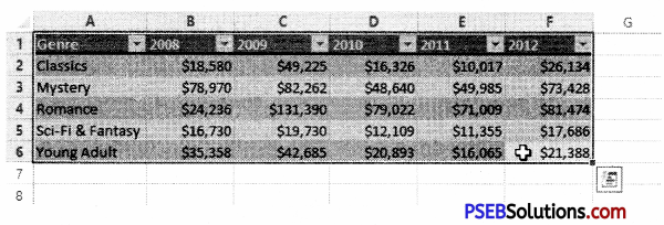
A chart is a tool that is used to communicate data graphically. A chart can allow knowing the meaning behind data.
Charts:
Excel has various types of charts, so we can choose one that most effectively represents our data.
![]()
Types of Chart:
- Pie Chart
- Column Chart
- Line Chart
- Bar Chart
- Area Chart
- Scatter Chart.
Create a Chart
To create a line chart, the steps are as follows:
1. Type the data in our excel worksheet.
2. Select the range.
3. On the Insert tab, in the Charts group, choose Line, and select Line with Markers.
![]()
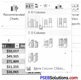
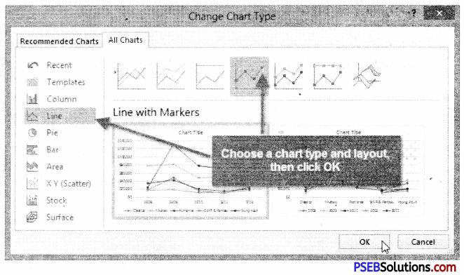
Change a chart type
We can easily change a chart type at any time. Following are the steps to change a chart type:
1. Select the chart.
2. On the Insert tab, in the Charts group, choose Column, and select Clustered Column.
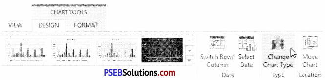
Switch Row/Column
1. Select the chart. Chart Tools contextual tab is activated.
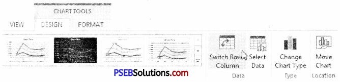
2. On the Design tab, click Switch Row/ Column.
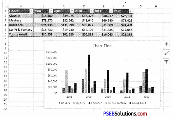
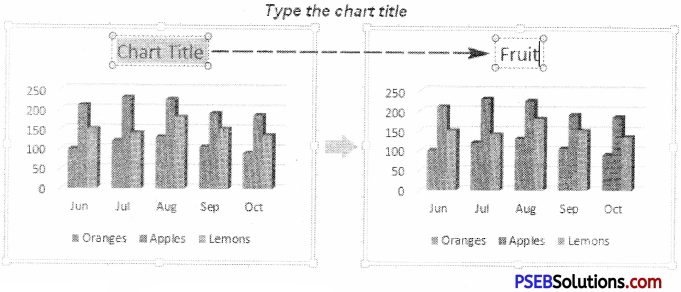
Add chart Title
1. Select the chart.
2. On the Layout tab, click Chart Title, Above Chart.
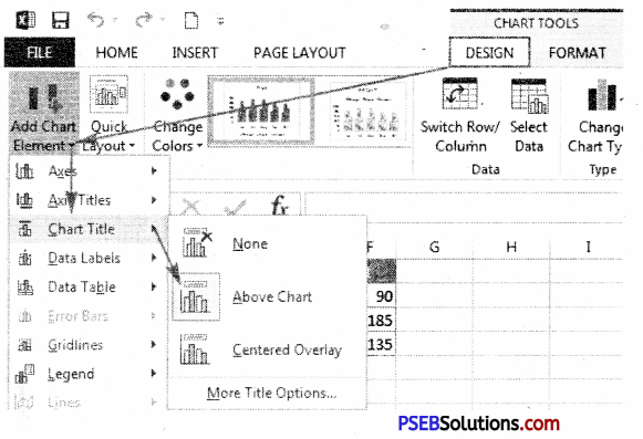
3. We will see a caption (Chart Title) above our chart. Enter our desired title.
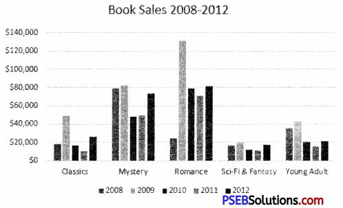
Elements of a Chart
- Chart area: A chart area contains everything inside the chart window, including all parts of the chart.
- Data marker: A data marker is a symbol on the chart that represents a single value in the worksheet. A data marker can be a bar in a bar chart, a pie in a pie chart, or a line on a line chart.
- Data series: It is a group of related values such as all the values in a single row in the chart.
- Axis: It is a line that is used as a major reference for plotting data in a chart.
- Tick mark: It is a small line intersecting an axis. A tick mark indicates a category, scale, or chart data series.
- Plot area: It is the area where our data is plotted and it includes the axes and all markers that represent data points.
- Gridlines: These are the optional lines extending from the tick marks across the plot area.
- Chart text: It is a label8- or title that we add to our chart. Attached text is a title or label that is linked to an axis such as the Chart Title.
- Legend: It is a key that identifies patterns, colors, or symbols associated with the markers of a chart data series. The legend shows the data series name corresponding to each data marker
![]()
Equations and Symbols
How to insert equations, symbols and special characters in excel:
Excel makes it easy to enter symbols, such as foreign currency marks, as well as special characters, like trademark and copyright symbols, into cells. These symbols are available in the Symbol dialog box.
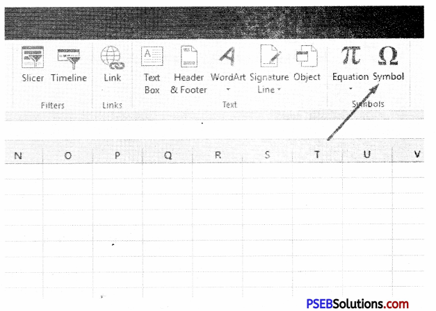
1. Click the Insert tab and then click the Symbol button in the Symbols group. The Symbol dialog box appears.
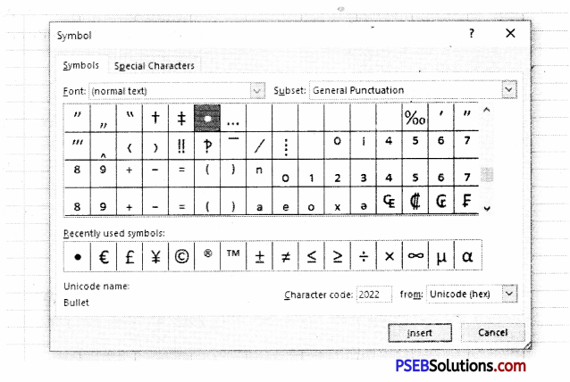
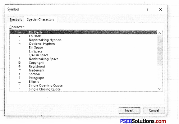
2. Select the desired symbol on the Symbols tab; or click the Special Characters tab and select the desired character.
3. Click Insert to insert the symbol or character.
4. Click close when we’re done adding symbols and special characters. The inserted symbols or characters appear in the worksheet.
5. Press Enter to complete the cell entry.
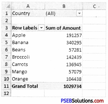
Pivot Table:
Insert Pivot Table
The data in a worksheet can be easily managed by using PivotTables. We can summarize the data. Pivot Table allows us to manipulate it in various ways. PivotTables are very helpful tool when we have to deal with large and complex spreadsheets.
A PivotTable is very helpful in doing these calculations. We can do calculations and summarize the data in a way that’s not only easy to read but also easy to manipulate.
![]()
How to create a PivotTable:
1. Select the table or cells – including column headers – containing the data we want to use.
2. From the Insert tab, click the PivotTable command.

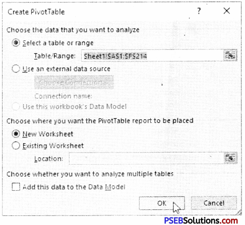
3. The Create PivotTable dialog box will appear. Click OK.
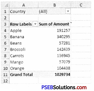
Add fields to the Pivot Table:
1. Before using Pivot Table, first of all we’ll need to decide which fields to add to the PivotTable. Each field is a column header from the source data.
2. In the Field List, place a check mark next to each field we want to add.
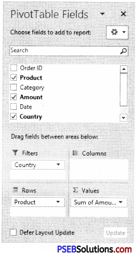
3. The selected fields will be added to one of the four areas below the Field List.
4. The PivotTable now shows the change.
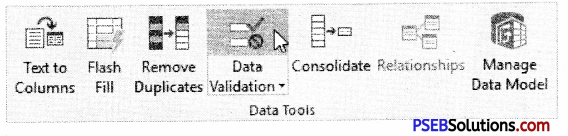
Data Tools:
Data Tools are simply tools which make it easy to manipulate data. Some of them are used to save our time by extracting or joining data and others perform complex calculations on data.
![]()
Convert Text to Columns:
Steps are as follows:
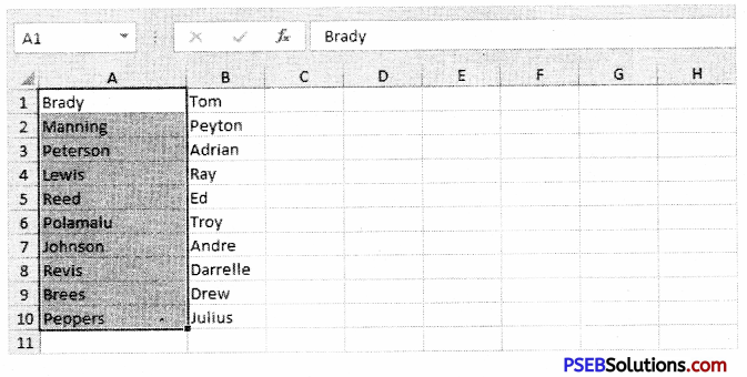
1. Type the data in our worksheet as:
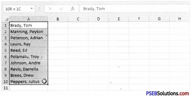
2. Select the range with full names.
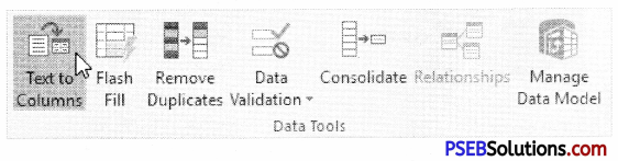
3. On the Data tab, click Text to Columns.
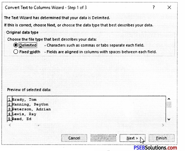
4. Choose Delimited and click Next.
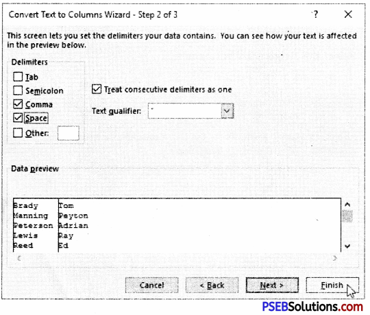
5. Clear all the check boxes under Delimiters except for the Comma and Space check box.
6. Click Finish.
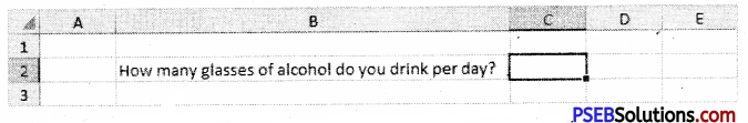
Data Validation:
Data validation is a powerful feature that is used to set up certain rules to dictate what can be entered into a cell.
![]()
How to Create Data Validation Rule:
To create a data validation rule, the steps are as follows:
1. Type the data in our excel worksheet.
2. Select cell D2.
3. On the Data tab, click Data Validation.
1. In the Allow list, click Whole number.
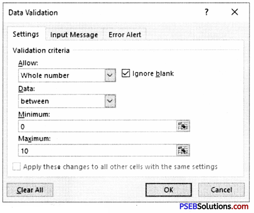
2. In the Data list, click between.
3. Enter the Minimum and Maximum values.
Input Message: Input messages appear when the user selects the cell and tell the user what to enter.
On the Input Message tabas below do the following:
1. Check ‘Show input message when cell is selected’.
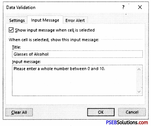
2. Enter a title.
3. Enter an input message.
Error Alert:
If users ignore the input message and enter a number that is not valid, we can show them an error alert.
On the Error Alert tab do the following:
1. Check ‘Show error alert after invalid data is entered1.
2. Enter a title.
3. Enter an error message.
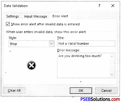
4. Click OK.
![]()
Data Validation Result:
To check our Data Validation result follows the steps as below:
1. Select cell C2.
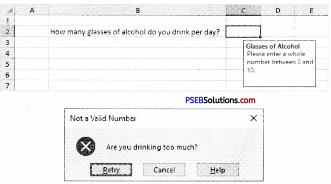
2. Try to enter a number higher than 10.
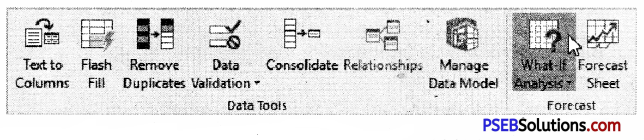
What-If Analysis:
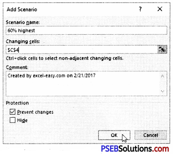
What-If Analysis in Excel allows us to try out different values (scenarios) for formulas. In MS Excel a scenario is a set of values that saves and can substitute automatically on our worksheet.
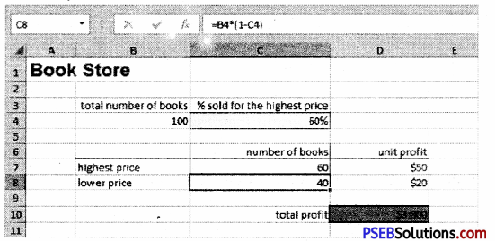
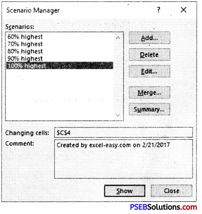
1. On the Data tab, click What-If Analysis and select Scenario Manager from the list.
2. The Scenario Manager Dialog box appears.
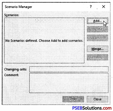
3. Type a name, select cell and click on OK.
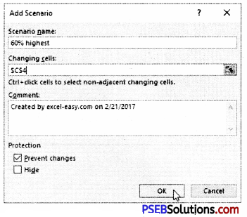
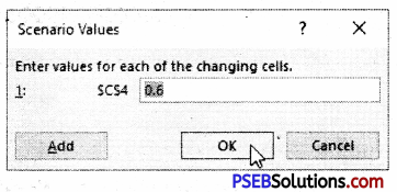
4. Enter the corresponding value and click on OK again.
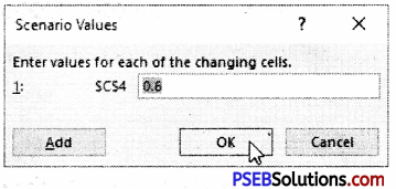
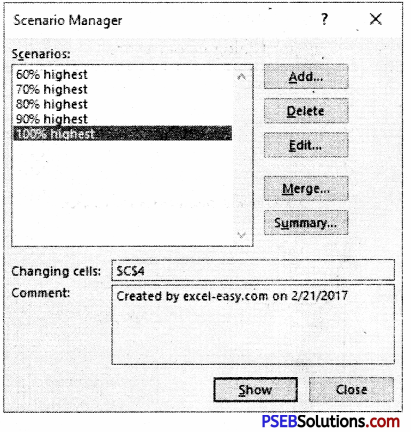
5. Next, add 4 other scenarios.
![]()
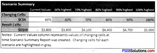
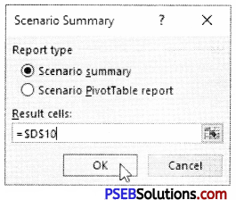
Scenario Summary:
After creating your required Scenarios, to easily compare the results of these scenarios following are the steps below:
1. Click the Summary button in the Scenario Manager.
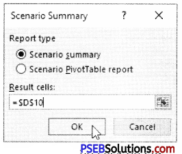
2. Next, select cell for the result cell and click on OK.
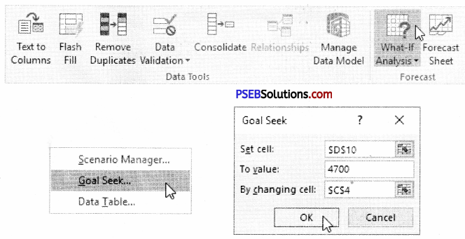
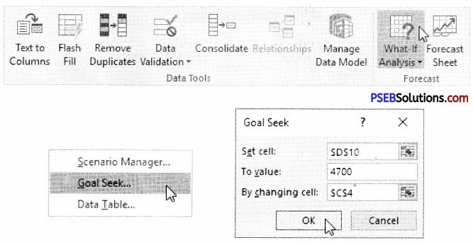
Goal Seek?
The goal seek function is a part of what-if analysis tool set. It allows a user to use the desired result of a formula to find the possible input value necessary to achieve that result.
3. Type a name, select cell and click on OK.
4. Enter the corresponding value and click on OK again.
5. Next, add 4 other scenarios.
Scenario Summary: After creating your required Scenarios, to easily compare the results of these scenarios following are the steps below:
1. Click the Summary button in the Scenario Manager.
2. Next, select cell for the result cell and click on OK.

Goal Seek?
The goal seek function is a part of what-if analysis tool set. It allows a user to use the desired result of a formula to find the possible input value necessary to achieve that result.
![]()
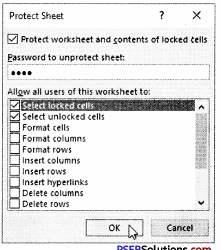
Protection:
In simple words Protection means to keep our stuff safe from misuse from an authorised person. In Excel we can protect our workbook/worksheet.
Protect Worksheet
Steps to Protect Worksheet:
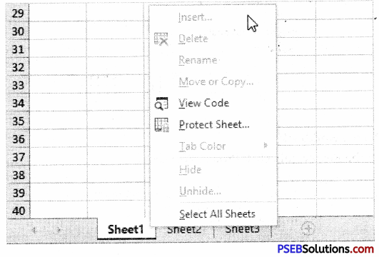
1. Right click a worksheet tab
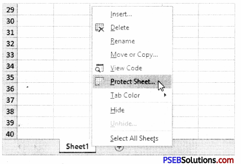
2. Click Protect Sheet.
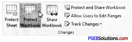
Protect Workbook
A workbook can be protected easily as we have protected a worksheet. A workbook can be protected such as:
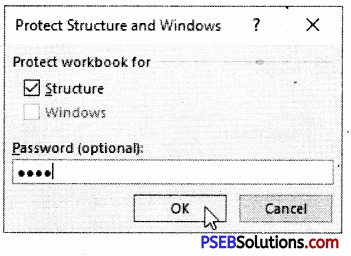
Structure: If we protect the workbook structure, users cannot insert, delete, rename, move, copy, hide or unhide worksheets anymore.
Windows: If we protect the workbook windows, we cannot move, change the size and close windows anymore.
1. Open a workbook.
2. On the Review tab, click Protect Workbook.
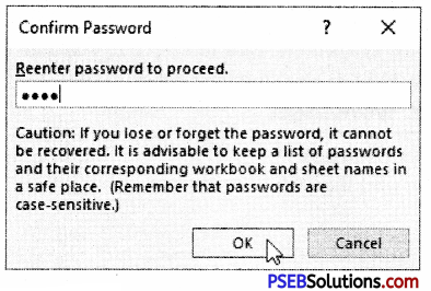
3. Check Windows enter a password and click OK.
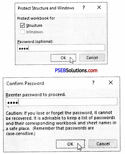
4. Re-enter the password and click on OK.
![]()
View Tab
Split
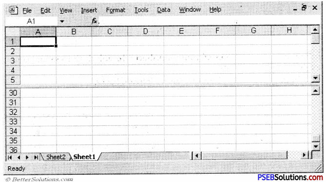
In Excel we can split the worksheet window into separate panes and scroll the worksheet in each pane so that we can easily compare data from two separate worksheet locations. We can make the panes in a workbook window disappear by double-clicking anywhere on the split bar that divides the window.
1. Click the split box above the vertical scroll bar.
2. Notice the two vertical scroll bars.
3. To remove the split, double click the horizontal split bar that divides the panes (or drag it up).
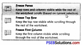
Freeze
Freeze option is very useful in some cases when we have a long table and want to see all. We need to scroll it while looking all the data. We will see that the table headings are also scrolled during scrolling, so it becomes difficult to understand the meaning of data without having its heading name hidden.
Freeze Top Row: To freeze the top row, execute the following steps.
1. On view tab, click Freeze Panes and then Freeze
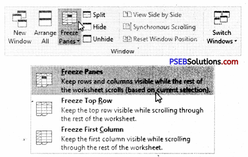
2. Scroll down to the rest of the worksheet.
![]()
How to Unfreeze Panes of your worksheet
To unlock all rows and columns, execute the following steps.
1. On the View tab, click Freeze Panes, Unfreeze Panes.
How to Freeze Panes of a Worksheet
To freeze panes, execute the following steps.
1. Select row.
2. On the View tab, click Freeze Panes, Freeze Panes.
3. Scroll down to the rest of the worksheet.
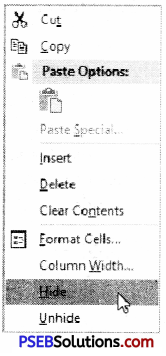
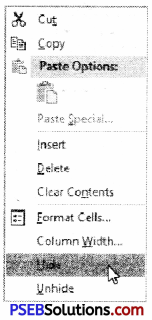
Hide/Unhide Columns, Rows and Sheets:
Hiding Rows:
In desired spreadsheet select the rows (for multiple selection hold Ctrl key and keep selecting) we want to hide and navigate to Home tab.
From Cells group, click Format button. Now from Hide & Unhide options, click Hide Rows.
Upon click it will automatically hide the selected rows.
![]()
Hiding Columns:
For hiding the columns in specific sheet, following are the steps:
1. Select the columns we want to handle.
2. Now click on Format button in Cells group. Now Click on Hide & Unhide options then click Hide Columns.
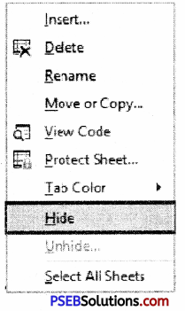
How to Hide Worksheets
Following are the steps to do so:
1. Select the sheet which we want to hide.
2. Now Click Hide Sheet from Hide & Unhide options from Cell group in Home Tab.
3. Click on Hinde Sheet Option from Hide and Unhide.
Macro:
A macro is a series of commands that is grouped together so that we can run whenever we need to perform the specific task. We can use macros in Excel to save time by automating tasks that we perform frequently.
The easiest method for creating many macros is to use macro recorder. When we record a macro Excel stores the information about each step you take as you perform a series of commands. We then run the macro to repeat or playback the set of commands.
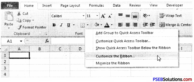
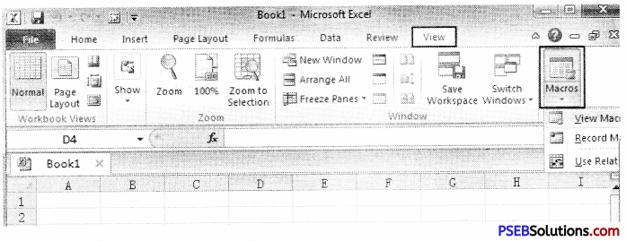
The macro recorder records every action we complete. So before we start the process of recording it is very important to plan macro- that what steps we need to record. To display the Developer tab, follow these steps:
1. Click the File tab and then click Options. The Excel Options dialog box
appears.
2. Click Customize Ribbon in the left pane, and then select the Developer check box under Main Tabs on the right side of the dialog box.
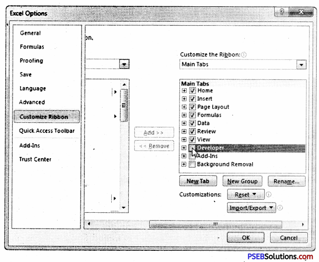
3. Click OK. The Developer tab appears in the Ribbon.
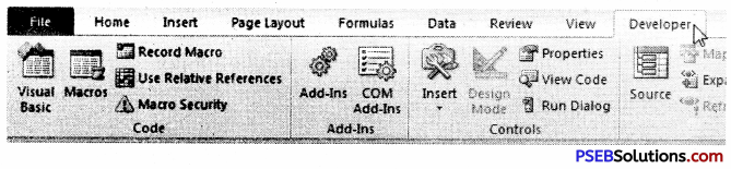
![]()
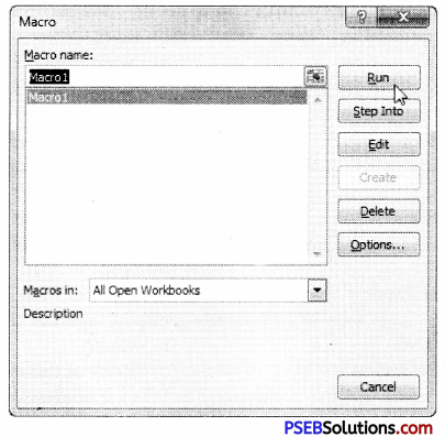
How to Record a macro:
Follow these steps to record a macro:
1. Choose Record Macro in the Code group of the Developer tab. The Record Macro dialog box appears.
2. Type a name for the macro in the Macro Name text box.
3. Assign a Shortcut Key.
4. From the Store Macro In drop-down list, select where we want to store the macro:
- This Workbook: Save the macro in the current workbook file.
- New Workbook: Create macros that we can run in any new workbooks created during the current Excel session.
- Personal Macro Workbook: Choose this-option if you want the macro to be available whenever we use Excel, regardless of which worksheet we’re using.
- Type a description of the macro in the Description text box.
- Click OK. The Record Macro option on the Developer tab changes to Stop Recording.
- Perform the actions you want to record.
- Choose Stop recording in the Code group of the Developer tab.
- The macro recorder stops recording keystrokes and the macro is complete.